R ggplot2: data visualiseren in R [tutorial & uitleg]

Grafieken met R package ggplot2

Binnen R is standaardfunctionaliteit aanwezig voor het maken van grafieken. Het kan echter voorkomen dat je ingewikkeldere grafieken wilt maken. In dat geval ben je al snel aangewezen op het R ggplot2 package.

De naam van ggplot2 staat voor Grammar of Graphics Plots en een goede documentatie is hier te vinden.

Dit blog is een onderdeel van een blogserie over R waarin we o.a. ingaan op hoe je R installeert, hoe je in RStudio werkt, hoe je datasets uitleest in R, data manipuleert met bijvoorbeeld dplyr of data.table.

In dit blog leer je meer over ggplot2 en visualisatie van data in R. Specifiek gaan we in op:

Data voorbereiden voor visualisatie in R
Structuur van grafieken met ggplot2
Labels bij R ggplot2 grafieken
Grafiektypes beschikbaar binnen ggplot2
Meerdere series in een ggplot2 grafiek
Grafiek opslaan met ggplot2

1. Data voorbereiden voor visualisatie in R

In deze tutorial werken we met datasets met KNMI metingen. Je kunt de datasets hier downloaden zodat je mee kunt doen met deze tutorial.

We bereiden enkele datasets voor vanuit de KNMI metingen om grafieken mee te maken.

1.1. Meetwaarden

library(readxl)
library(dplyr)
library(lubridate)

df_knmi <- read_excel("data/knmi_measurements.xlsx", guess_max = 10000)

df_knmi <- df_knmi %>%
  mutate(temperature = temperature / 10) %>%
  mutate(date = as.Date(as.character(date), format = "%Y%m%d")) %>%
  mutate(month = month(date)) %>%
  mutate(year = year(date)) %>%
  mutate(decennium = floor(year(date) / 10) * 10) %>%
  mutate(station_id = as.character(station_id))

df_knmi

## # A tibble: 275,935 × 7
##    station_id date       temperature rainfall month  year decennium
##    <chr>      <date>           <dbl>    <dbl> <dbl> <dbl>     <dbl>
##  1 260        1901-01-01        -4.9       NA     1  1901      1900
##  2 260        1901-01-02        -1.8       NA     1  1901      1900
##  3 260        1901-01-03        -2.6       NA     1  1901      1900
##  4 260        1901-01-04        -6.5       NA     1  1901      1900
##  5 260        1901-01-05        -6         NA     1  1901      1900
##  6 260        1901-01-06       -10         NA     1  1901      1900
##  7 260        1901-01-07        -9.2       NA     1  1901      1900
##  8 260        1901-01-08        -4.9       NA     1  1901      1900
##  9 260        1901-01-09         1.1       NA     1  1901      1900
## 10 260        1901-01-10         1.5       NA     1  1901      1900
## # ℹ 275,925 more rows

Ook interessant: clean dataset in R: hoe ga ik te werk?

1.2. Gemiddelde meetwaarden per maand

df_month <- df_knmi %>%
  group_by(month) %>%
  select(month, temperature, rainfall) %>%
  summarise(
    mean_temperature = mean(temperature, na.rm = TRUE),
    mean_rainfall = mean(rainfall, na.rm = TRUE)
  )

df_month_station <- df_knmi %>%
  group_by(month, station_id) %>%
  select(month, station_id, temperature, rainfall) %>%
  summarise(
    mean_temperature = mean(temperature, na.rm = TRUE),
    mean_rainfall = mean(rainfall, na.rm = TRUE)
  )

df_month_station

## # A tibble: 144 × 4
## # Groups:   month [12]
##    month station_id mean_temperature mean_rainfall
##    <dbl> <chr>                 <dbl>         <dbl>
##  1     1 240                    3.07          20.8
##  2     1 260                    2.48          21.5
##  3     1 267                    3.13          21.0
##  4     1 269                    3.32          21.5
##  5     1 279                    2.89          23.5
##  6     1 283                    2.89          21.5
##  7     1 286                    2.61          21.1
##  8     1 290                    2.07          22.7
##  9     1 310                    3.56          19.3
## 10     1 340                    3.69          18.6
## # ℹ 134 more rows

df_month

## # A tibble: 12 × 3
##    month mean_temperature mean_rainfall
##    <dbl>            <dbl>         <dbl>
##  1     1             2.87          21.2
##  2     2             3.16          19.0
##  3     3             5.66          17.2
##  4     4             8.77          14.2
##  5     5            12.7           18.0
##  6     6            15.5           21.8
##  7     7            17.4           24.6
##  8     8            17.3           25.6
##  9     9            14.5           23.3
## 10    10            10.8           23.8
## 11    11             6.51          23.9
## 12    12             3.81          24.1

Met vertrouwen waardevolle inzichten halen uit data met R? Bekijk dan onze opleiding R voor data analyse.

1.3. Gemiddelde meetwaarden per decennium

df_decennium <- df_knmi %>%
  group_by(decennium) %>%
  select(decennium, temperature, rainfall) %>%
  summarise(
    mean_temperature = mean(temperature, na.rm = TRUE),
    mean_rainfall = mean(rainfall, na.rm = TRUE)
  )

df_decennium_station <- df_knmi %>%
  group_by(decennium, station_id) %>%
  select(decennium, station_id, temperature, rainfall) %>%
  summarise(
    mean_temperature = mean(temperature, na.rm = TRUE),
    mean_rainfall = mean(rainfall, na.rm = TRUE)
  )

df_decennium_station

## # A tibble: 89 × 4
## # Groups:   decennium [13]
##    decennium station_id mean_temperature mean_rainfall
##        <dbl> <chr>                 <dbl>         <dbl>
##  1      1900 260                    8.70          19.6
##  2      1900 310                    9.34         NaN  
##  3      1900 380                    8.65         NaN  
##  4      1910 260                    9.09          22.4
##  5      1910 310                    9.96         NaN  
##  6      1910 380                    9.08         NaN  
##  7      1920 260                    8.91          19.8
##  8      1920 310                    9.90         NaN  
##  9      1920 380                    9.13         NaN  
## 10      1930 260                    9.35          21.0
## # ℹ 79 more rows

df_decennium

## # A tibble: 13 × 3
##    decennium mean_temperature mean_rainfall
##        <dbl>            <dbl>         <dbl>
##  1      1900             8.84          19.6
##  2      1910             9.37          22.4
##  3      1920             9.31          19.8
##  4      1930             9.64          21.0
##  5      1940             9.48          20.7
##  6      1950             9.50          20.6
##  7      1960             9.27          22.9
##  8      1970             9.52          19.2
##  9      1980             9.63          21.1
## 10      1990            10.0           21.5
## 11      2000            10.6           22.6
## 12      2010            10.6           21.2
## 13      2020            10.5           20.9

2. Structuur van grafieken met ggplot2

Iedere ggplot2 grafiek bevat 3 componenten:

Dataset
Visuele configuratie (dit wordt aesthetic mapping genoemd)
Grafiektype (dit wordt geometry genoemd)

Zie het volgende voorbeeld. We starten met (1) alleen een canvas voor de dataset:

library(ggplot2)

ggplot(
  data = df_month,  ## Dataset
)

We gaan door met (2) een configuratie van de data (aesthetic mapping):

ggplot(
  data = df_month,  ## Dataset
  mapping = aes(x = month, y = mean_temperature)  ## Aesthetic mapping
)

Tenslotte voegen we een (3) grafiektype toe (geometry):

ggplot(
  data = df_month,  ## Dataset
  mapping = aes(x = month, y = mean_temperature)  ## Aesthetic mapping
) + 
  geom_line()  ## Geometry

3. Labels bij R ggplot2 grafieken

Met de labs() functie kun je labels toevoegen zoals voor:

Assen
Titel
Subtitel

Zie onderstaand voorbeeld:

ggplot(
  data = df_decennium,
  mapping = aes(x = decennium, y = mean_temperature)
) + 
  geom_point() +
  labs( 
    title = "Average temperature development in the Netherlands", 
    subtitle = "Temperatures in degrees Celcius", 
    y = "Temperature [°C]", 
    x = "Year",
    caption = "Source: KNMI"
  )

4. Grafiektypes bij R ggplot2 grafieken

We bekijken verschillende grafiektypes.

4.1. Lijngrafiek

Met functie geom_line() kun je een lijngrafiek (line chart) maken:

ggplot(
  data = df_decennium,
  mapping = aes(x = decennium, y = mean_temperature)
) + 
  geom_line(color = "dodgerblue") +
  labs( 
    title = "Average temperature development in the Netherlands", 
    subtitle = "Temperatures in degrees Celcius", 
    y = "Temperature [°C]", 
    x = "Year",
    caption = "Source: KNMI"
  )

4.2. Staafgrafiek

Met functie geom_col() kun je een staafgrafiek (bar chart) maken:

ggplot(
  data = df_decennium,
  mapping = aes(x = decennium, y = mean_temperature)
) + 
  geom_col(fill = "dodgerblue") +
  labs( 
    title = "Average temperature development in the Netherlands", 
    subtitle = "Temperatures in degrees Celcius", 
    y = "Temperature [°C]", 
    x = "Year",
    caption = "Source: KNMI"
  )

4.3. Histogram

Met functie geom_histogram() kunnen we een histogram maken:

ggplot(
  data = df_knmi,
  mapping = aes(x = temperature)
) + 
  geom_histogram(fill = "dodgerblue") +
  labs( 
    title = "Histogram of daily temperatures in the Netherlands", 
    subtitle = "Temperatures in degrees Celcius", 
    y = "Count", 
    x = "Temperature [°C]",
    caption = "Source: KNMI"
  )

4.4. Boxplot

Met functie geom_boxplot() kunnen we een boxplot maken:

ggplot(
  data = df_knmi,
  mapping = aes(x = reorder(as.character(month), month), y = temperature)
) + 
  geom_boxplot() +
  labs( 
    title = "Average temperature by month in the Netherlands", 
    subtitle = "Temperatures in degrees Celcius", 
    y = "Temperature [°C]", 
    x = "Year",
    caption = "Source: KNMI"
  )

4.5. Heatmap

Met functie geom_tile() kun je een heatmap maken:

We gebruiken functie scale_fill_gradient() om de kleuren in te stellen.
We gebruiken geom_text() om de waarden te tonen.


ggplot(
  data = df_decennium_station,
  mapping = aes(
    x = as.character(decennium),
    y = as.character(station_id),
    fill = mean_temperature
  )
) + 
  geom_tile() +
  scale_fill_gradient(high = "red", low = "yellow") + 
  geom_text(aes(label = round(mean_temperature, 1))) +
  labs( 
    title = "Average temperature development in the Netherlands by station", 
    subtitle = "Temperatures in degrees Celcius", 
    y = "Station", 
    x = "Year",
    caption = "Source: KNMI",
  )

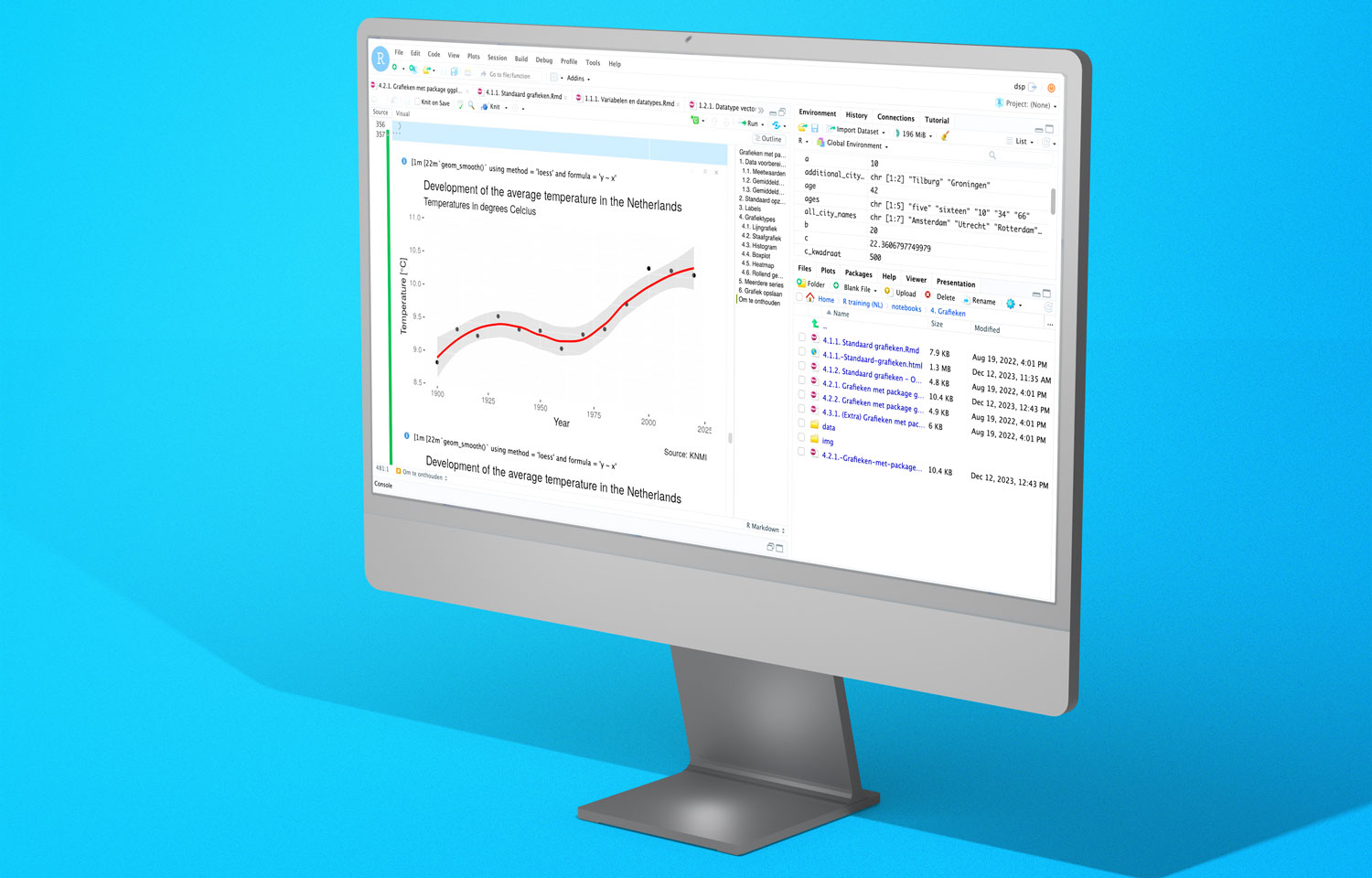
4.6. Rollend gemiddelde

Door een rollend gemiddelde toe te voegen zie je gemakkelijk eventuele trends.

We doen dit met functie geom_smooth():

ggplot(
  data = df_decennium,
  mapping = aes(x = decennium, y = mean_temperature)
) + 
  geom_point() +
  geom_smooth(color = "red") +
  labs( 
    title = "Development of the average temperature in the Netherlands",
    subtitle = "Temperatures in degrees Celcius", 
    y = "Temperature [°C]", 
    x = "Year",
    caption = "Source: KNMI"
  )

Je ziet hier standaard ook het 95% betrouwbaarheidsinterval.

5. Meerdere series in een ggplot2 grafiek

In onderstaand voorbeeld bekijken we meerdere series in 1 grafiek.

Hierbij plotten we de gemiddeld maandelijkse temperatuur voor ieder weerstation.

We maken gebruik van parameter color:

Met functie scale_x_continuous() stellen we de waarden op de x-as in.

ggplot(
  data = df_month_station,
  mapping = aes(
    x = month,
    y = mean_rainfall,
    color = station_id
  )
) + 
  geom_line() + 
  geom_point() +
  labs( 
    title = "Average daily rainfall by month by KNMI weather station", 
    subtitle = "Rainfall in millimeters",
    y = "Rainfall [mm]", 
    x = "Month",
    caption = "Source: KNMI",
    color = "Station"
  ) +
  scale_x_continuous(breaks = 1:12)

6. Grafiek opslaan met ggplot2

Met functie ggsave() sla je een grafiek op:


ggplot(
  data = df_decennium,
  mapping = aes(x = decennium, y = mean_temperature)
) + 
  geom_col() +
  labs( 
    title = "Development of the average temperature in the Netherlands",
    subtitle = "Temperatures in degrees Celcius", 
    y = "Temperature [°C]", 
    x = "Year",
    caption = "Source: KNMI"
  )

ggsave(
  filename = "data/output/temperature_by_decennium_bar_ggplot2.png"
)

## Saving 7 x 5 in image

Je kunt de grafiek nu opzoeken in de map data/output

Expert worden in R?

Wil jij goed leren werken in R? Tijdens onze Opleiding R leer je alles wat je nodig hebt om zelfstandig analyses uit te voeren in R.

Rik van der Wardt

Rik is data scientist en marketeer bij Data Science Partners. Vanuit zijn achtergrond op de Technische Universiteit Eindhoven heeft hij veel affiniteit met data. Na zijn studie heeft hij als consultant altijd met data gewerkt en tevens ervaring opgedaan in het geven van trainingen.